Synchronizing on Strings and String interning

I’ve  recently had to solve a problem of synchronizing a piece of code on some String objects in Java. Here’s a short description: “In a network management system, you need to handle different events produced for different IPs. Code must support multithreading, but if more events are generated at the same time for the same IP,  you must handle those events in original order, one at a time. IPs are stored as String objects”.

Now, let’s say the method signature is public void process(String ip, Event event). It’s obvious that you shouldn’t make the entire method synchronized because it won’t be multithreaded anymore. The first thing that might come to your mind can be to add a block like synchronized(ip) { … process event … } . Please note that String objects are immutable and, for the same IP  value (eg. “11.111.11.1”), you might have two different String objects. So, synchronizing on ip directly would not be a good idea.

What you might not know is that Java supports String interning : “a method of storing only one copy of each distinct string value, which must be immutable. Interning strings makes some string processing tasks more time- or space-efficient at the cost of requiring more time when the string is created or interned. The distinct values are stored in a string intern pool.”  The corresponding method in Java is String.intern()  which checks if the string pool contains a value equal to the String object for which the method is called as determined by the String.equals(Object) method. If  String object is found, the method returns the reference to the object from the pool. If string not found, then it’s first added to the pool and a reference is returned.

Java automatically interns String literals. This means that in many cases, the == operator appears to work for Strings in the same way that it does for ints or other primitive values, but it is strongly recommended to use String.equals(Object) method (which by the way is first checking if object references are the same). The intern()  method is to be used on Strings constructed with new String(). Here are some examples of String interning:

String s1 = "test";
String s2 = "test";
String s3 = "test".intern();
String s4 = new String("test");
String s5 = new String("test").intern();

String result = "Testing String interning: \n";
result += (s1 == s1) ? "s1 and s2 are identical \n" : ""; // true
result += (s1 == s3) ? "s1 and s3 are identical \n" : ""; // true
result += (s1 == s4) ? "s1 and s4 are identical \n" : ""; // false
result += (s1 == s5) ? "s1 and s5 are identical \n" : ""; // true

There are some disadvantages of interning strings:

  1. you must ensure that intern() method is called for all the strings (except string literals or constants) that you’re going to compare. Someone using your code might forget to intern strings and confusingly results might be returned.
  2. intern() calls are quite expensive because it has to manage the pool of strings

So, please make sure you know what you are doing before starting using interning.

Going back to our problem, String interning can help us synchronizing on IPs. Here’s how our method should look like:

public void process(String ip, Event event) {
    // ...
    synchronized(ip.intern()) {
        // process event
    }
    // ...
}

You might think everything is fine with this piece of code, but, by interning a String, it turns into a global object and if you’re synchronizing on the same interned string in different parts of your application, you can end up with deadlocks. There’s a small probability for this to happen, but you must take it into account that anybody can add a piece of code like that outside your module and you won’t even notice it.
Appending HTML fragment to a DOM Element

The common solution for appending an HTML fragment like ‘<li><span>Element 1</span></li><li><a href=”url”>Click me</a></li>’ to an UL element is to create and add each node by hand:

var item = document.createElement('LI');
var span = document.createElement('SPAN');
span.appendChild(document.createTextNode('Element 1'));
item.appendChild(span);

ul.appendChild(item);

Maybe you are asking why not appending the fragment to UL‘s innerHTML like:

ul.innerHTML += '<li>Element 1</li><li><a href="url">Click me</a></li>';

The next example will answer to your question:

<ul id="persistentEventTest">
	<li>Element 1</li>
	<li>Element 2</li>
</ul>
-------------------------------------
var list = document.getElementById('persistentEventTest');
var items = list.getElementsByTagName('LI');

for (var i = 0, len = items.length; i < len; i++) {
items[i].addEventListener('click', function () {console.log('Why did you click ME?');}, false);
}

//list.innerHTML += '<li>I will break it!</li>';

You can test it here.
If you uncomment the last line, you won’t be able to trigger the ‘click’ events on LI elements because when you modify the innerHTML for any DOM element, all the attached listeners will be lost!

A faster and more elegant solution is the one from here :

var container = document.createElement('DIV');
container.innerHTML = '<li>Element 1</li><li><a href="url">Click me</a></li>';
while (container.firstChild)
     ul.appendChild(container.firstChild);

So, you need to create a new container, add the fragment to it as innerHTML and then you can add his children to the desired target. In this way, no existing listeners will be removed.

The only fishy part might be:

while (container.firstChild)
     ul.appendChild(container.firstChild);

Why does this work if no ‘removeChild’ function is called ?
Actually, when you call ‘appendChild()’ for a child which is a reference to an existing node in the document, then the function moves it from its current position to the new one.

So, there’s no reason to explicitly remove it.

iPhone Viewport Scaling

According to Mobile Statistics, Stats & Facts 2011, by 2014, mobile internet will take over desktop internet usage. And that’s not hard to believe taking into account the 1.08 bilion smart-phones on the market.
So, let’s suppose you own a smartphone. Then you have certainly navigated to a not mobile friendly webpage and you needed to zoom for making the text readable.

You probably know that zooming can be activated using the ‘viewport’ metadata.
<meta name="viewport" content="width=device-width; initial-scale=1.0; maximum-scale=2.0; user-scalable=1;" />

However, changing an iOS device orientation from portrait to landscape causes the page to scale larger than 1.0 and a part of the page (right) will be cropped. This effect will disappear if the user double-taps the screen, but lots of users don’t know about this trick.

The simplest solution would be to deactivate the zoom on your web-page by using the same value for ‘maximum-scale’ and ‘initial-scale’ or by setting ‘user-scalable’ to ‘0’ (on iOS you must use ‘no’ instead of ‘0’):
<meta name="viewport" content="width=device-width; initial-scale=1.0; maximum-scale=1.0; user-scalable=1;" />

But this won’t make the page easy to read on mobile devices. So, let’s try to find a fix for iOS.
Using media queries, you can write something like this:

@media screen and (orientation:landscape) and (device-width:320px) and (device-height: 480px) {
	body {
		width: 480px;
	}
}

which should force the browser to set the width to 480px (the resolution for iOS devices) on landscape. This rule should apply only for iPhone. If there are other devices with the same resolution, they won’t be affected because the 480px will be used anyway.

This rule might look OK, but there’s actually a bug on iOS which returns the same width (320px) for portrait and landscape and you can’t forced it to other values.
That’s pretty strange because Apple knows about this old bug, but they still sustain that’s the intended behavior. Why ? Probably they want to copy MS with their crazy IE exceptions. 😀

These being said, there’s only one solution left: to use JavaScript.
So, we can deactivate the zoom on iPhone when the page is loaded using the method explained above (same values for ‘initial-scale’ and ‘maximum-scale’) and activate it when the user starts making a gesture. Zoom will be activated by setting ‘initial-scale’ to 0.25 and ‘maximum-scale’ to 1.6 (default values from Apple’s Oficial document).
The original solution can be found here.

/**
 * Fix viewport when device orientation is changed and zoom is enabled
 */
function fixViewport(doc) {
	var event = 'gesturestart',
	    qsa = 'querySelectorAll',
	    scales = [1, 1], //initial scale width and height
	    meta = qsa in doc ? doc[qsa]('meta[name=viewport]') : [];

	function fix() {
		meta.content = 'width=device-width,minimum-scale=' + scales[0] + ',maximum-scale=' + scales[1];
		doc.removeEventListener(event, fix, true);
	}

	if ((meta = meta[meta.length - 1])) {
		fix();
		// enable zoom when gestures start
		scales = [.25, 1.6];
		doc.addEventListener(event, fix, true);
	}
};
function init() {
	//...
	if (navigator.userAgent.match(/iPhone|iPod|iPad/))
		fixViewport(document);
	//...
}

window.addEventListener("load", init, false);

The code searches in page metadata tags and modifies the ‘viewport’ metadata by setting the ‘initial-scale’ and ‘maximum-scale’ to 1.0 (deactivates zoom). When a ‘gestureStart’ event takes place, the zoom is reactivated.
In this way, the scaling bug is fixed and the user will still be able to zoom. Also, this fix won’t impact other mobile browsers which have correctly implemented scaling.

Decision Trees – C4.5

C4.5 is an algorithm developed by Ross Quinlan that generates Decision Trees (DT), which can be used for classification problems. It improves (extends) the ID3 algorithm by dealing with both continuous and discrete attributes, missing values and pruning trees after construction. Its commercial successor is C5.0/See5, a lot faster that C4.5, more memory efficient and used for building smaller decision trees.

Being a supervised learning algorithm, it requires a set of training examples and each example can be seen as a pair: input object and a desired output value (class). The algorithm analyzes the training set and builds a classifier that must be able to correctly classify both training and test examples. A test example is an input object and the algorithm must predict an output value (the example must be assigned to a class).

The classifier used by C4.5 is a decision tree and this tree is built from root to leaves by respecting the Occam’s Razor. This razor says that given two correct solution for a certain problem, we should choose the simpler solution.

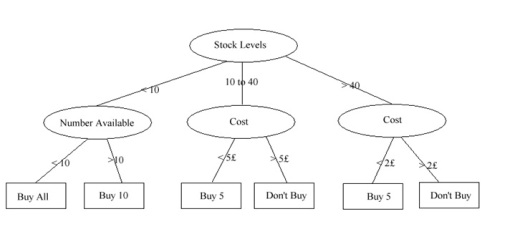
Here is an example of a decision tree built using C4.5:

The input and output requirements and a pseudo-code for the C4.5 algorithm is presented below:

The input for the algorithm consists of a set S of examples described by continuous or discrete attributes, each example belonging to one class.

The output is a decision tree or/and a set of rules that assigns a class to a new case (example).

Algorithm:

Check for base case.
Find the attribute with the highest informational gain (A_best)
Partition S into S1,S2,S3... according to the values of A_best
Repeat the steps for S1,S2,S3...
<em>

The base cases are the following:

•  All the examples from the training set belong to the same class ( a tree leaf labeled with that class is returned ).

•  The training set is empty ( returns a tree leaf called failure ).

•  The attribute list is empty ( returns a leaf labeled with the most frequent class or the disjuction of all the classes).

The attribute with the highest informational gain is computed using the following formulas:

Entropy:  E(S ) = \sum_{i=1}^{n}-Pr(C_i)*log_2Pr(C_i)
Gain:  G(S,A) = E(S)-\sum_{i=1}^mPr(A_i)E(S_{Ai})

E(S) – information entropy of S

G(S,A) – gain of S after a split on attribute A

n – nr of classes in S

Pr(Ci) – frequency of class Ci in S

m – nr of values of attribute A in S

Pr(Ai) – frequency of cases that have Ai value in S

E(SAi) – subset of S with items that have Ai value

The C4.5 algorithm improves the ID3 algorithm by allowing numerical attributes, permitting missing values and performing tree pruning.

Numeric attributes:

Temperature attribute:

In order to deal with attributes like temperature (may have a lot of numerical values) binary split is performed. The values of the attribute are sorted. Then, the gain is computed for every split point of an attribute. It is chosen the best split point (h) and  the Ai attribute is split like this: Ai ≤ h, Ai > h.

An optimal binary split is done when it is evaluated the gain only between points of different classes. For example, we don’t have to evaluate the gain between 72 and 75 because they are assigned to the same class ‘Yes’ and this point will surely not be chosen for split. In addition to this, we should not repeat the order of the values at each node, because the order for a node’s children can be determined from the order of the values of the parent.

Missing values:

Missing values are usually marked with “?”. Dealing with missing values involves imputation. Imputation means that if an important feature is missing, it can be estimated from the available data.

Distribution-based imputation is done when we split the example into multiple instances, each with a different value for the missing feature. It is assigned a weight corresponding to the estimated probability for the particular missing value and the weights sums up to 1.

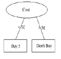
For example: Split the 18 instances by Cost: 10 go down the <5Ł branch, 8 down the >5Ł branch. So when  we get an instance without Cost, the classification for <5Ł happened 10/18 times and the classification for >5Ł, 8/18 times. We can say that ‘Buy 5’ has 5/9 ‘votes’ and ‘Don’t buy’ 4/9 ‘votes’. So, instead of having a single class assigned to an example, we have more classes and each class has a certain probability. Most likely, we will choose as correct the class with the highest probability.

Tree pruning:

Tree pruning is done in order to obtain smaller trees and avoid over-fitting (the algorithm tries to classify the training data so well and it becomes too specific to correctly classify the test data).

Pruning can be done in two ways: pre-pruning and post-pruning. With pre-pruning we stop building the tree when the attributes are irrelevant. It is harder to perform, but faster. When post-pruning we build the entire tree and remove certain branches. We can do this by either using sub-tree raising or sub-tree replacement.

C4.5 algorithm performs sub-tree replacement. This means that a sub=tree is replaced by a leaf if it reduces the classification error.

We estimate error rate as follows: suppose a node classifies N instances with E errors. Then, the actual error rate on new cases usually higher than E/N.

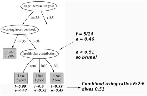
One way of estimating the error rate is by splitting the training set and estimate errors according to the instances not used for training. Another way is by performing pessimistic pruning (we increases the number of errors observed at each node). We base our increase on the error rate on training set, number of instances convered by node and confidence level. If the combined error for a set of branches is higher than the parent, prune them.

Example of tree pruning using pessimistic pruning:

Advantages & disadvantages:

The advantages of the C4.5 are:

•  Builds models that can be easily interpreted

•  Easy to implement

•  Can use both categorical and continuous values

•  Deals with noise

The disadvantages are:

•   Small variation in data can lead to different decision trees (especially when the variables are close to each other in value)

•  Does not work very well on a small training set

Conclusion

C4.5 is used in classification problems and it is the most used algorithm for builing DT.

It is suitable for real world problems as it deals with numeric attributes and missing values. The algorithm can be used for building smaller or larger, more accurate decision trees and the algorithm is quite time efficient.

Compared to ID3, C4.5 performs by default a tree pruning process, which leads to smaller trees, more simple rules and more intutive interpretations.

BackPropagation NN

As you already know from the previous article, BackPropagation is a supervised learning algorithm for feed-forward neural networks. The network doesn’t need feedback.

After initializing the neurons weights with random values between two values, the network is capable to automatically adjust the weights using a two phase algorithm:

  • ˆforward propagation of a training pattern’s input through the neural network to activate the neurons and get the network outputs
  • back propagation from the outputs node to the inner ones in which phase the network previous outputs are compared with the expected outputs from the training patterns, an error estimation is computed and back propagated in order to adjust neurons weights.

The network has an input layer, one or more hidden layers and an output layer.
The number of neurons on each layer can be adapted to meet the requirements.
A neuron is an entity that copies the human brain neuron. It responds to a given input based on the activation function and weights. If the activation function’s output is greater than a threshold, the neuron is excited (it produces an output).
In order to be considered valid, the neuron’s activation function must be di fferentiable.
Being a gradient descent method, it minimizes the total squared error of the output computed by the net.

The aim is to train the network to achieve a balance between the ability to respond correctly to the input patterns that are used for training and the ability to provide a good response to the inputs that are similar.

The main steps for training the network are:

initialize neurons weights randomly in [ -1 ,1]
while not all examples have been classified correctly
    for each example E in the training set
         forward phase -> compute network's output Out
         error = expected output - Out
         compute delta for all weights backward
         update weights
return network

The sigmoid function is the most used in neuron’s activation step:
f(x) = \frac{1}{1+e^{-x}}

A hidden neuron’s (neuron on a hidden layer) output (h) is calculated using the next formula:
h_{j} = f(\sum_{i=1}^{A} w_{hij}x_i - \theta_j) , j = 1..B
where x_i are the network inputs, w_{ij} are the weights, \theta is the activation function threshold, A the inputs number and B the hidden neurons number.The output layer results are calculated using this formula:
y_{j} = f(\sum_{i=1}^{B} w_{oij}h_i - \theta_j) , j = 1..C
where h_i was calculated before and C is the output layer’s neurons number.
The errors for the output layer and for the hidden layer are computed with:
\delta_{oj} = y_j(1-y_j)(d_j-y_j), j = 1..C
\delta_{hj} = h_j(1-h_j)\sum_{i=1}^{C} w_{ij}\delta_{oi}, j = 1..B
where d_j is the network expected output.The weights for the next step are adjusted as follow:
w_{oij}(t+1) = \eta\delta_{oj}h_i+w_{oij}(t), i = 1..B, j = 1..C
w_{hij}(t+1) = \eta\delta_{hj}x_i+w_{hij}(t), i = 1..A, j = 1..B
where \eta is the learning rate.

Using the interfaces presented in the ANN Introduction article, I implemented a basic BackPropagation Network. Here’s the source code for the Neuron:

/**
 * Neuron used in BackPropagation Neural Network
 * @author Octavian Sima
 */
public class BackPropagationNeuron implements Neuron<Double> {

 private int inputsNumber;         //number of neuron inputs
 private Double[] inputs;          //neuron inputs
 private Double[] weights;         //neuron weights
 private Double biasWeight;        //bias neuron weight
 private Double output;            //neuron output after calling compute
 private BackPropagationNetwork parent;  //network which contains the neuron

 @Override
 public void initNeuron(NeuralNetwork<Double> parent, int inputsNumber,
         Double initialWeightMinValue, Double initialWeightMaxValue) {

     this.initialWeightMinValue = initialWeightMinValue;
     this.initialWeightMaxValue = initialWeightMaxValue;
     this.initNeuron(parent, inputsNumber);
 }

 @Override
 public void initNeuron(NeuralNetwork<Double> parent, int inputsNumber) {
     this.parent = (BackPropagationNetwork)parent;
     this.inputsNumber = inputsNumber;
     this.inputs = new Double[inputsNumber];
     this.weights = new Double[inputsNumber];
     //generate random weights for neuron predecesors
     this.generateRandomWeights();
 }

 @Override
 public double activationFunction(Double value) {
     //sigmoid function = 1/(1+e^-x)
     return 1.0 / (1.0 + Math.exp(-1.0 * value));

     //asinh function = ln(x+sqrt(x^2+1))
     //return Math.log(value + Math.sqrt(value * value + 1));
 }

 @Override
 public double activationFunctionDerivative(Double value) {
     //sigmoid function derivative = value * (1 - value)
     return value * (1-value);

    //asinh function derivative = 1/sqrt(1+x^2)
    //return 1/Math.sqrt(1+ value * value);
 }

 @Override
 public Double compute(Double[] input) {
     //forward phase - propagate the output
     Double total = 0.0;
     //update inputs and compute output
     for (int i = 0; i < this.inputsNumber; i++) {
         this.inputs[i] = input[i];
         total += this.weights[i] * input[i];
     }
     //add bias
     total += this.biasWeight;

     //apply activationFunction
     this.output = this.activationFunction(total);
     return this.output;
 }

 /**
 * Backward phase - neuron learns (adjust its weights) from error
 * @param error   error used in weights adjusting
 */
 public void adjustWeights(double error) {
     for (int i = 0; i < this.inputsNumber; i++) {
         double delta = error * this.inputs[i] * this.parent.getLearningRate();
         this.weights[i] += delta;
     }
     //adjust bias neuron weight
     this.biasWeight += error * this.parent.getLearningRate();
 }

 /**
 * Generate random weights between initialWeightMinValue and initialWeightMaxValue
 */
 private void generateRandomWeights() {
     //Random rand = new Random();
     for (int i = 0; i < this.inputsNumber; i++) {
         this.weights[i] = 0.2 * (Math.random() - 0.5);
     }
     this.biasWeight = 0.2 * (Math.random() - 0.5);
 }

 public double getOutput() {
     return this.output;
 }

 public double getWeight(int neuronIndex) {
     return this.weights[neuronIndex];
 }
}

You should be able to use the NeuralNetwork interface in order to implement the BackPropagation network. If you have difficulties, write your email and I’ll send you the code.

Artificial Neural Networks (ANN) – Introduction

An Artificial Neural Network is an emulation of the more complex biological neural system. Why do we need such an abstract model ? Although computing performances reached these days are very high, there are certain tasks that a common microprocessor is unable to perform. In some of these cases, the ANN approach can provide better results.

Biological Neural Network

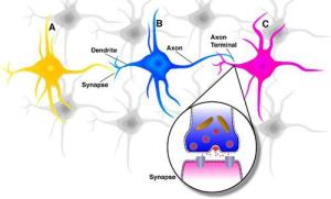
You can see how our brain is structured.  A huge number of neurons are interconnected using their synapses. A neuron is activated  when the sum of its inputs (electrical signals) is greater than a threshold.  If a neuron is activated, it produces an output (another electrical signal) which is propagated in the network. No reaction(inhibition)  means no electrical signal.

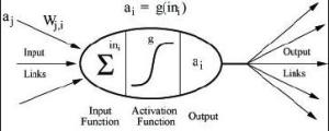
This model can be easily copied in Computer Science. Take a look at the next images:

Brain neuronArtificial neuron

Now, we can give a better definition for ANN:  a group of simple and identical computing units (strong related to biological neurons) which operates in parallel being able to perform complex tasks. Each link between two neurons has a weight associated with. We can say that the weights  represent the neural network’s knowledge.

This approach has a lot of advantages, but also some disadvantages.

ANN advantages:

  • Fault tolerance: when an element/group of elements or links of the neural network fail, the network’s performance, in most of the cases, won’t be affected.
  • Adaptive learning (from examples)
  • A neural network learns and does not need to be reprogrammed.
  • A neural network can perform tasks that a linear program can not.
  • Real-time operating after the learning process is finished (due to the parallel structure)
  • Self organizing capacity: an ANN can create its own  organization and representation of data during the training process.
  • ANN can be implemented in any application without a great effort. Once you have your own ANN source, many problems can be mapped.

Disadvantages:

  • The neural network needs training to operate and, sometimes, training data is not available.
  • The architecture of a neural network is different from the architecture of microprocessors therefore needs to be emulated.
  • Requires high processing time for large neural networks.

For a better understanding of the way an ANN works, let’s  analyze the mathematical model of a neuron.

mathematical model of a neuron

The synapses of the neuron are modeled as weights. The strength of the connection between an input and a neuron is noted by the value of the weight. Negative weight values reflect inhibitory connections, while positive values designate excitatory connections [Haykin].

An adder sums up all the inputs modified by their respective weights.

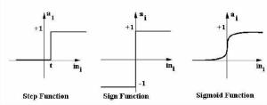
The activation function controls the amplitude of the output of the neuron. An acceptable range of output is usually between 0 and 1, or -1 and 1.

A well-known activation function is the Threshold Function which takes on a value of “0” if the summed input is less than a certain threshold value  and the value “1” if the summed input is greater than or equal to the threshold value.

The sigmoid function uses the formula : f(t) = 1 / (1 + e^-t).

Activation functions graphics can be seen below.

activation functions

It’s important to distinguish three types of units (neurons):

  • input neurons  (i) – receive data from outside the neural network
  • output units (o) – send data out of the neural network
  • hidden units (h) whose input and output signals remain within the neural network.

During training, the weights can be updated either synchronously or asynchronously.

There are two types of neural network topologies:

  • Feed-forward neural networks, where the data flow from input to output units is strictly feed-forward, no feedback is provided for any training step.
  • Feedback networks, where the network’s output (from a training step) is backward propagated in order to update neurons weights. The most representative networks for this category are the Back-Propagation Networks, which I will detail in the next article.

The training process can be performed using

  • supervised learning – learning from a set of examples – the network is trained by providing it with input and matching output patterns
  • unsupervised learning – or self-organizing neural networks – the system must develop its own representation of the input stimuli because there is no classified set of examples to learn from. A well-known unsupervised network is SOM (Self-Organizing Map) which can be used in many domains to group (cluster) similar units. I will dedicate a new article for this type of ANN.

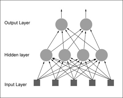
Finally, let’s see how an ANN looks like:

Neural Network example

Notice that the Middle Layer is called the Hidden Layer and we can have a different number of neurons on each layer and also a different number of hidden layers. Actually, there is no rule for choosing these numbers, you will have to discover by yourself what’s the best configuration for the problem you want to solve.

This method of “tuning” is used in every Machine Learning algorithm and it consists in changing different constants and running the algorithm on different data sets and finally choosing the best values.

Also, you should already know that every link from the previous image has a weight associated with. The final scope of the training phase is to set the right weights (usually initiated with small random numbers).

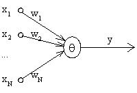
The Perceptron is  the simplest neural network. Actually, it is less than a neural network, it is a computational unit with a threshold value (Theta) which, for x1,x2,…xn inputs and w1,w2,…wn weights, it produces an +1 output if the sum of wi*xi (for i=1,N) is >= Theta and 0 (or -1) output otherwise.

Perceptron

Perceptron

The Perceptron divides the inputs space into 2 areas (one for points with +1 output, and one for points with 0 output).

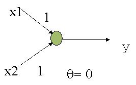
A limitation of the Perceptron is that it can only compute linearly separable functions like the OR function:

OR-function

OR function using a Perceptron

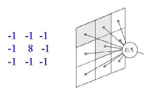
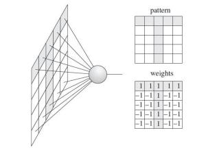
But, even with such a primitive network, we can perform interesting tasks like edge detection, corner detection and even character recognition (using pattern matching). Here are some examples:

Corner-detection

Corner detection

Character recognition

Character recognition

These are the Neuron and NeuralNetwork Java interfaces which I’ll implement in the next article for the BackPropagation Neural Network. You are free to use them and you can try to implement a Perceptron to recognize the T letter.

/**
 * Neuron representation for NeuralNetwork algorithm
 * @param     type of data used by network
 * @author Octavian Sima
 */
public interface Neuron {

 /**
 * Initialize neuron
 * @param parent                    network which contains the neuron
 * @param inputsNumber              number of neuron inputs
 * @param initialWeightMinValue     minValue used in initial weight computing
 * @param initialWeightMaxValue     maxValue used in initial weight computing
 */
 void initNeuron(NeuralNetwork parent, int inputsNumber,
 E initialWeightMinValue, E initialWeightMaxValue);

 /**
 * Initialize neuron with default values
 * @param parent            network which contains the neuron
 * @param inputsNumber      number of neuron inputs
 */
 void initNeuron(NeuralNetwork parent, int inputsNumber);

 /**
 * Neuron reaction (computes the output generated by an input array)
 * @param input       input dataset
 * @return            output value
 */
 E compute(E[] input);

 /**
 * Neuron activation function
 * @param value
 * @return
 */
 double activationFunction(E value);

 /**
 * ActivationFunction first derivate
 * @param value
 * @return
 */
 double activationFunctionDerivative(E value);
}
/**
 * NeuralNetwork template
 * @param     type of data used by network
 * @author Octavian Sima
 */
public interface NeuralNetwork {

 /**
 * Initialize neural network
 * @param layersNumber            network's number of layers
 * @param neuronsNumberOnLayer    array with number of neurons on each layer
 * @param learningRate            neuron learning rate
 * @param learnCalmingRate        calming rate of learningRate(1.0 - constant)
 */
 void initNetwork(int layersNumber, int neuronsNumberOnLayer[],
 double learningRate, double learnCalmingRate);

 /**
 * Initialize neural network with default values
 * @param layersNumber            network's number of layers
 * @param neuronsNumberOnLayer    array with number of neurons on each layer
 */
 void initNetwork(int layersNumber, int neuronsNumberOnLayer[]);

 /**
 * Train network on a given data set
 * @param inputs            inputs data set
 * @param outputs           expected results
 * @param maxAcceptedError  maximum accepted error for training phase to stop
 * @param maxSteps          maximum number of steps in training
 * @return                  number of steps really used in training before convergence
 */
 int train(E[][] inputs, E[][] outputs, double maxAcceptedError, int maxSteps);

 /**
 * Train network on a given data set with default maxSteps
 * @param inputs            inputs data set
 * @param outputs           expected results
 * @param maxAcceptedError  maximum accepted error for training phase to stop
 * @return                  number of steps really used in training before convergence
 */
 int train(E[][] inputs, E[][] outputs, double maxAcceptedError);

 /**
 * Test network on a given input
 * @param input       input data
 * @return            result
 */
 E[] test(E[] input);
}

WWW ?

Who?

I should begin with presenting myself:  I’ve graduated Computer Science and, in present, I attend a Master in Artificial Intelligence.

What?

I’ve created this blog in order to teach you some basic things in the fields  of Artificial Intelligence, Machine Learning and Computer Vision.

Why?

I hope that you’ll understand the importance of those algorithms in Computer Science domain and maybe you’ll be able to improve one or more of them.